JMP

One-Way

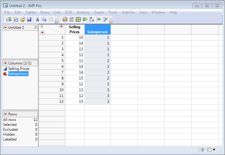
1. Enter all of the data into Column 1, one column at a time.

2. Under Cols, choose New Columns…

3. In the New Column window that opens, click the dropdown beside Modeling Type. Select Nominal. Select OK.

   

4. Enter the groups into Column 2 for each data value. Label the columns as fitting.

   

5. Under Analyze, choose Fit Y by X.

6. Click on the name of your data in Column 1 in the Select Columns box and click Y, Response. Click on the name of your data in Column 2 in the Select Columns box and click X, Factor. Select OK.

   

7. In the window that opens, click on the Red Triangle and select Means/Anova.

   

Tukey's HSD

1. Enter the data for the treatments in one column of an open JMP data table and a column for the response variable in another column and label the columns accordingly.

   

2. Select Analyze in the top row of the JMP spreadsheet and then select Fit Y by X.

3. From the Select Columns box, click on your treatments, then click on X, Factor. Click on your response and then click on Y, Response. Click OK.

   

4. From the Oneway Analysis output, click on the red triangle next to Oneway Analysis of…, then click on Compare Means and select All Pairs, Tukey HSD. The results of the test are displayed.

   

Note: You can adjust the α level by clicking the red triangle next to Oneway Analysis of… and then select Set α Level.

Two-Way

1. Enter all of the data into Column 1, one column at a time.

2. Under Cols, choose New Columns…

3. In the New Column window that opens, click the dropdown beside Modeling Type. Select Nominal. Select OK. Repeat this step to add a third column.

4. Enter the row names into Column 2 and the column numbers into Column 3. Label the columns as fitting.

5. Under Analyze, choose Fit Model.

6. Click on the name of your data in Column 1 in the Select Columns box and click Y. Highlight the names of your data in Column 2 and Column 3 at the same time in the Select Columns box. Click Macros and then Full Factorial. Select Run.

   

Test for Association

1. With a JMP Data Table open, enter the categories appearing in the rows of the contingency table into Column 1 and the categories appearing in the columns of the contingency table into Column 2, repeating categories to include all intersections of rows and columns from the contingency table. Enter the appropriate frequencies for each contingency table cell in Column 3.

   

2. Choose Analyze from the top row of the JMP spreadsheet, select Fit Y by X.

3. From the Select Columns box click on the variable in Column 1 and then and click Y, Response. Then, click on the variable in Column 2 in the Select Columns box and then click X, Factor. From the Select Columns box click on the variable for Frequency (in Column 3) and click Freq. Click OK.

   

4. Observe the results in the new window. Note: The second row (labeled “Pearson”) under Test in the output corresponds to the methods used in the texts.

Test for Goodness of Fit

1. With a JMP Data Table open, enter the categories in Column 1 and the actual (observed) frequencies in Column 2. Type in column headers.

   

2. Choose Analyze from the top row of the JMP spreadsheet, and then select Distribution.

3. From the Select Columns box, click on the column 1 variable and then click Y, Columns. From the Select Columns box, select your Actual Frequency (Observed) column and then click Freq. Click OK.

   

4. In the new window, select the Red Triangle next to the variable name. Select Test Probabilities.

   

5. Enter the hypothetical probabilities (Expected) under Hypoth Prob. Click Done.

   

6. Observe the results at the bottom of the window. Note: The second row (labeled “Pearson”) under Test in the output corresponds to the methods used in the texts.

   

Minimum Sample Size

1. Under DOE, click Design Diagnostics, and then Sample Size and Power. In the window that opens, select one of the situations listed. For this example, click One Sample Mean.

2. Enter your σ-level (the default value is 0.05) in the box Alpha, the standard deviation in the box Std Dev, the margin of error in the box Difference to detect, and 0.5 in the box Power. Click Continue. The sample size needed for this set of input values will display in the Sample Size box.

   

Proportion

1. Enter the data into the worksheet.

   

2. Choose Analyze, Distribution.

3. Select your variable in the Select Columns box. Click Y, Columns. Select your Frequency column and click Freq. Click OK.

   

4. Select the Red Triangle beside your variable name. Select Confidence Interval, and then your confidence level. If your confidence level is not present, select Other and then type your confidence level.

   

Note: JMP calculates confidence intervals for proportions using the score method.

Standard Deviation

1. Enter the data into Column 1 of the JMP data table.

2. Choose Analyze, Distribution.

3. Select your variable in the Select Columns box. Click Y, Columns. Click OK.

   

4. Select the Red Triangle beside your variable name. Select Confidence Interval, and then your confidence level. If your confidence level is not present, select Other and then type your confidence level.

   

5. The confidence interval for the standard deviation is shown in the second row of the Confidence Intervals table at the bottom of the output.

   

t-Interval

1. Enter the data into the worksheet.

2. Choose Analyze, Distribution.

3. Select your variable in the Select Columns box. Click Y, Columns. Click OK.

   

4. Select the Red Triangle beside your variable name. Select Confidence Interval, and then your confidence level. If your confidence level is not present, select Other and then type your confidence level.

   

Two Sample Proportions z-Interval

1. Enter the data into two columns with the grouping variable in Column 1 and the response variable in Column 2.

   

2. Under Analyze, choose Fit Y by X.

3. Click on the name of your data (Column 2) in the Select Columns box and click Y, Response. Click on the groups of your data (Column 1) in the Select Columns box and click X, Factor. Select OK.

   

4. In the window that opens, click on the Red Triangle and select Two Sample Tests for Proportions.

   

Two Sample t-Interval (Dependent Samples, Paired Difference)

1. Enter the data for the first sample in Column 1 of a JMP table and the data for the second sample in Column 2.

   

2. Select Analyze, Specialized Modeling, and then Matched Pairs.

3. From the Select Columns box, click on Column 1, then click on Y, Paired Response. Click on Column 2, then click on Y, Paired Response. Click OK.

   

4. By default, JMP produces a 95% confidence interval for the mean difference. To change the confidence level, click on the red triangle next to Matched Pairs, click on Set α Level and select 0.01. The results are displayed.

   

Variance

1. Enter the data into the worksheet

2. Choose Analyze, Distribution.

3. Select your variable in the Select Columns box. Click Y, Columns. Click OK.

   

4. Select the Red Triangle beside your variable name. Select Confidence Interval, and then your confidence level. If your confidence level is not present, select Other and then type your confidence level.

   

5. Right click on the table below Confidence Intervals. Select Make into Data Table.

6. In the new data table that opens, under Cols, select New Columns Name the column Lower CI Squared. Click Column Properties, then Formula.

   

7. In the new window that opens, click on Lower CI. Click x^y. Click OK twice.

   

8. Repeat Steps 6 and 7, naming the new column Upper CI Squared and clicking Upper CI instead of Lower CI.

9. The values in the row labeled Std Dev under the Lower CI Squared and Upper CI Squared columns are the lower and upper limits for the confidence interval for the variance.

   

z-Interval

1. Enter the sample mean or raw data into Column 1. If you enter a sample mean, enter the sample size into Column 2.

2. Choose Analyze, Distribution.

3. Select Column 1 in the Select Columns box. Click Y, Columns. Select Column 2 if you entered a mean and sample size in Step 1 and click Freq. Click OK.

   

4. Select the Red Triangle beside your variable name. Select Confidence Interval, and then select Other. Type your confidence level and check the box labeled Use Known Sigma. Click OK.

   

5. Enter your known standard deviation in the box that opens. Click OK.

   

One Variable

1. Enter the data into Column 1 of the worksheet.

2. Choose Analyze, Distribution.

3. Click Column 1 in the Select Columns box. Click Y, Columns. Click OK.

   1. To select additional statistics to be displayed in the Summary Statistics box, click the Red Triangle beside Summary Statistics and then select Customize Summary Statistics. Select the desired statistics you want to be displayed and click OK.

      

Two Variable

1. Enter the data into the worksheet, one variable in each column.

2. Choose Analyze, Distribution.

   

3. Click your first column in the Select Columns box. Hold the Ctrl key and click your second column in the Select Columns box. Click Y, Columns. Click OK.

   1. To select additional statistics to be displayed in the Summary Statistics box, click the Red Triangle beside Summary Statistics and then select Customize Summary Statistics. Select the desired statistics and click OK. You will have to repeat this process for both variables.

Critical Value

1. With a JMP Data Table open, click in the first cell of Column 1. Click on Cols in the top row and then select New Columns.

2. In the popup window that opens, click on Column Properties at the bottom of the window. Select Formula from the dropdown menu.

3. Click on the arrow next to Probability and select F Quantile. The F Quantile formula will appear.

   

4. To find the F-distribution critical value with 0.95 area to the left (or 0.05 area to the right) with 12 numerator degrees of freedom and 16 denominator degrees of freedom, input 0.95 for p, 12 for dfnum, and 16 for dfden. Press Enter.

5. Click Apply and then OK in the first window. The formula with the values displayed for p, dfnum, and dfden will appear at the bottom of the second window. Click Apply and then OK.

6. The value of 2.4246600017 should appear in row 1 of Column 2. If the value does not appear then double-click in the first row to the left of Column 2.

   

Bar Charts

1. In a JMP worksheet, enter the data with categories in Column 1 and numerical values in Column 2.

2. Choose Graph from the top row of the JMP display and select Graph Builder.

3. From the 2 Columns box drag and drop the variable in Column 1 to the drop zone along the horizontal axis. Repeat this action with the Column 2 variable and the vertical axis. Select the Bar Chart icon from along the top of the window.

   

4. Press Done to display the graph.

   

Choropleth Map (County)

1. In a JMP worksheet, download a data set containing geographical data. Note: For this example, we will use the US County Data found on the Hawkes Companion Website.

2. For JMP to match the data to a map shape, the region variable should be configured as a five-digit string, including leading zeroes. If the data is not currently in this format, as is the case in the US County Data data set, proceed with the following instructions:

   1. From the top row of the JMP spreadsheet, select Cols and then New Columns to create a column to store the new format.

   2. In the Column name window type “fips5”. In Data type choose “Character”.

   3. In Number of columns to add section, select Before first column from the dropdown menu.

   4. From the Column Properties dropdown menu select Formula and then Edit Formula.

      

   5. In the leftmost column of the new window, select Character and then Right.

      

   6. First click in the box labeled “text” and then in the leftmost column, select Character and then Concat.

      

   7. In the formula display, click the box to the left of the two vertical lines. Select Character, and then Char from the leftmost column. Type “0” (including the quotation marks) in the box. Press Enter.

      

   8. In the formula display, click the box to the right of the two vertical lines. From the list of columns in the data set, click on the column which contains the region strings.

      

   9. In the formula display, click in the box containing n. Type 5. Press Enter. Press OK twice.

      

   10. In the data set a new column is created, fips5, that is now configured with a leading zero.

       

3. Choose Graph from the top row of the JMP display and then select Graph Builder.

4. Click and drag the column containing the new 5-digit region variable to the Map Shape drop zone in the lower left corner of the Chart Area.

   

5. From the list in the window on the left, select the column which contains the data to be displayed in the graph and then click the Color button on the right of the screen. Press Done to display the graph.

   

6. Right click on the column name in the legend area to display the Legend Settings window. Type the title of the chart into the Title window. The color display can be adjusted when you select Color Theme. Make a choice and then select OK. Press OK.

   Note: To display the legend using the sequential gradient, in this data set we defined the variable type for Column 9 to be Numeric.

   

7. Press Done to display the map.

   

Dot Plot

1. In a JMP worksheet enter the data in a column.

2. Choose Graph from the top row of the JMP display, then select Graph Builder.

3. Click and drag the variable to the drop zone along the horizontal axis. From the Jitter dropdown menu choose Positive Grid.

   

4. Press Done to display graph. To adjust the vertical size of the window drag the horizontal axis up to desired height.

   

Histogram

1. In a JMP worksheet, enter the data into a column.

2. Choose Analyze from the top row of the JMP display. Select Distribution.

3. From the Select Columns box, click on the variable and then click Y, Columns. Click OK.

   

4. In the new window, click on the red triangle beside the variable name and select Display Options, Horizontal Layout.

   

5. To adjust the class width, click the red triangle beside the variable name and select Histogram Options, Set Bin Width. Enter your desired class width and click OK.

   
   

Line Graphs

1. With a JMP Data Table open, enter the data with the variables in Column 1 and Column 2. Include column headers to be displayed as axis titles in the graph.

2. Choose Graph from the top row of the JMP spreadsheet, and then select Graph Builder.

3. From the 2 Columns box click and drag a variable to the drop zone along the horizontal axis. Repeat this action with the other variable and the vertical axis.

4. Select Line Graph icon from options along the top of the Graph Builder window.

   

5. Click Done to display the graph.

   

Multivariate/Multinomial

1. With a JMP Data Table open, enter the data with one variable in each column.

2. Choose Graph from the top row of the JMP spreadsheet, and then select Bubble Plot.

3. In the Select Columns box, choose the desired y-variable and then click the Y button. In the Select Columns box, choose the desired x-variable and then click the X button. In the Select Columns box, choose the desired variable for size of the bubbles and then click Sizes. Note: Additionally, using Coloring will further distinguish the variable used for Sizes.

   

4. Press OK to display graph. To adjust the size of the bubbles use the slider shown in bottom left corner.

   

Normal Probability Plot

1. In a JMP worksheet, enter the data into Column 1.

2. Choose Analyze from the top row of the JMP display. Select Distribution.

3. Click Column 1 in the Select Columns box. Click Y, Columns. Click OK.

   

4. In the new window, click on the red triangle beside the variable name and select Display Options, then Horizontal Layout.

   

5. Click on the red triangle beside the variable name and select Normal Quantile Plot.

   

Pareto Chart

1. Enter the data into the worksheet, one variable in each column.

2. Under Analyze, click Quality and Process, and then Pareto Chart.

3. Click the column containing your categories in the Select Columns box and click Y, Cause. Click the column containing your data values in the Select Columns box and click Freq.

   

4. Click OK.

Pie Chart

1. Enter the data into the worksheet, one variable in each column.

2. Choose Graph from the top row of the JMP spreadsheet, and then select Graph Builder.

3. From the 2 Columns box click and drag the column 1 categories to the drop zone along the horizontal axis. Repeat this action with the column 2 variable using the vertical axis.

4. Select the Pie Chart icon from the options along the top of the Graph Builder window.

   

5. To display labels on the pie chart, select from the Label dropdown menu in the Graph Builder window.

   

6. Click DONE to display the graph.

   

Scatterplot

1. Enter the data into the worksheet, one variable in each column.

2. Under Analyze, click Fit Y by X.

3. Click the column containing your suspected independent variable in the Select Columns box and click X, Factor. Click the column containing your suspected dependent variable in the Select Columns box and click Y, Response. Click OK.

   

Stem-and-Leaf Plot

1. Enter the data into Column 1 of a new data table.

2. Under Analyze, click Distribution.

3. Click your variable in the Select Columns box and click Y, Columns. Click OK.

   

4. Click the red triangle beside your variable name in the window that opens. Click Stem and Leaf.

   

Paired Difference

1. Enter the data into the worksheet, one variable in each column.

2. Under Analyze, click Specialized Modeling, and then Matched Pairs.

3. Select each of the two variables in the Select Columns box and then click Y, Paired Response. Click OK.

   

4. To adjust the significance level of the test, click the red triangle beside Matched Pairs and then click Set σ Level. Choose your desired level. The test results will display at the bottom of the window.

   

z-Test

If Raw Data is Available:

1. Enter the data into the worksheet in Column 1.

2. Click Analyze, and then click Distribution.

3. Select Column 1 in the Select Columns box and then click Y, Columns. Click OK.

   

4. Click the red triangle beside your variable name. Click Test Mean.

   

5. Enter the hypothesized mean, and the population standard deviation. Click OK.

   

If Summary Statistics are Available:

1. Click Help, and then Sample Data.

2. Under Teaching Resources, click the arrow beside Calculators, and then click Hypothesis Test for One Mean.

   

3. Select Summary Statistics and click OK.

   

4. Select z-test. Select the type of test based on the alternate hypothesis. Enter the values for the hypothesized mean, sample average, population standard deviation, sample size, and significance level (alpha). Click the box labeled Reveal Decision. The test results will populate in the bottom right of the open dialog box.

   

t-Test

If Raw Data is Available:

1. Enter the data into the worksheet in Column 1.

2. Click Analyze, and then click Distribution.

3. Select Column 1 in the Select Columns box and then click Y, Columns. Click OK.

   

4. Click the red triangle beside your variable name. Click Test Mean.

   

5. Enter the hypothesized mean. Click OK.

   

If Summary Statistics are Available:

1. Click Help, and then Sample Data.

2. Under Teaching Resources, click the arrow beside Calculators, and then click Hypothesis Test for One Mean.

   

3. Select Summary Statistics and click OK.

   

4. Select t-test. Select the type of test based on the alternate hypothesis. Enter values for the hypothesized mean, sample average, sample standard deviation, sample size, and significance level (alpha). Click the box labeled Reveal Decision. The test results will populate in the bottom right of the open dialog

   

Two Proportion z-Test

1. Click Help, and then Sample Data.

2. Under Teaching Resources, click the arrow beside Calculators, and then click Hypothesis Test for Two Proportions.

   

3. Select Summary Statistics and click OK.

   

4. Select the type of test based on the alternate hypothesis. Enter the hypothesized difference (the default value is 0), sample 1 count, sample 1 size, sample 2 count, sample 2 size and significance level (alpha). Click the box labeled Reveal Decision. The test results will populate in the bottom right of the open dialog box.

   

Two Sample z-Test

1. Click Help, and then Sample Data.

2. Under Teaching Resources, click the arrow beside Calculators, and then click Hypothesis Test for Two Means.

   

3. Select Summary Statistics and click OK.

   

4. Select z-test and the type of test based on the alternate hypothesis. Enter the corresponding statistics in the Test Inputs boxes. Click the box labeled Reveal Decision. The test results will populate in the bottom right of the open dialog box.

   

Kruskal-Wallis Test

1. With a JMP Data Table open, enter the data for each sample in a separate column of the table and label them accordingly.

   

2. Select Table in the top row, and then Stack. From the Select Columns box, click on each sample then click on Stack. Make sure Stack By Row is selected. Click OK.

   

3. Select Analyze in the top row of the JMP output table, then select Fit Y by X. From the Select Columns box, click on Data, then click on Y, Response. Click on Label and then click on X, Factor. Click OK.

   

4. From the output, click on the red triangle next to Oneway Analysis of…. Click on Nonparametric and select Wilcoxon Test.

   

Spearman Rank Correlation Test

1. With a JMP Data Table open, enter the data for each variable in a separate column of the table and label them accordingly.

   

2. Select Analyze in the top row of the JMP output table, then select Multivariate Methods and then Multivariate. From the Select Columns box, click on each variable, then click on Y, Response. Click OK.

   

3. From the output, click on the red triangle next to Multivariate. Click on Nonparametric Correlations and select Spearman's p.

   

Wilcoxon Rank-Sum Test

1. With a JMP Data Table open, enter the data for the response variable in one column of the table and the variable containing the group label into another column of the table.

   

2. Click on Analyze in the top menu. Then select Fit Y by X.

3. Click on the response variable in the Select Columns and click Y, Response. Click on the group variable name and click X, Factor. Click OK.

4. From the Oneway Analysis output, click on the red triangle next to Oneway Analysis of…, then click on Nonparametric and select Wilcoxon Test. The first table of output displays the sum of the ranks and the mean rank for each group. The test statistic and p-value for the test are in the table labeled 2-Sample Test.

   

Wilcoxon Signed Rank Test

1. With a JMP Data Table open, enter the data for the paired responses in two different columns of the JMP table and label them accordingly.

   

2. Select Analyze in the top row of the JMP output table, then select Specialized Modeling and then Matched pairs. From the Select Columns box, select both data columns. Then select Y, Paired Response. Note: 2008(x) must be selected first to perform 2006 – 2008. Click OK.

   

3. From the output, click on the red triangle next to Matched Pairs and select Wilcoxon Signed Rank. The output for the test is shown below.

   

Test for Normality

1. With a JMP Data Table open, enter the data into Column 1 and label it appropriately.

   

2. Select Analyze in the top row of the JMP output table, and then select Distribution. From the Select Columns box, click on Column 1, then click on Y, Response. Click OK.

3. From the output, click on the red triangle next to Column 1. Click on Continuous Fit and select Fit Normal. Then, click on the red triangle next to Fitted Normal Distribution and select Goodness of Fit. Note: To get the output to show horizontally, click on the red triangle next to Column 1 and choose Display Options and Horizontal Layouts.

   

Critical Value

1. With a JMP Data Table open, click in the first cell of Column 1. Click on Cols in the top row and then select New Columns.

2. In the popup window that opens, click on Column Properties at the bottom of the window. Select Formula from the dropdown menu.

3. Click on the arrow next to Probability and select Tukey HSD Quantile. The Tukey HSD Quantile formula will appear.

   

4. To find the q-distribution critical value with α = 0.05 , 3 groups (or treatments) and 147 degrees of freedom, input 0.95 for 1 - alpha, 3 for nGroups, and 147 for dfe. Press Enter.

5. Click Apply and then OK in the first window. The formula with the values displayed for 1 - alpha, nGroups, and dfe will appear at the bottom of the second window. Click Apply and then OK.

6. The value of 2.3677316411 should appear in row 1 of Column 2. If the value does not appear then double-click in the first row to the left of Column 2.

   

7. The value given is an adjusted value. Multiply this value by $\sqrt{2}$ to get the q-distribution critical value of 3.348.

Linear Regression Fitted Line Plot with Confidence Interval

1. Enter your data in the worksheet.

2. Click Analyze and Fit Y by X.

3. Select the y-variable in the Select Variables box. Click Y, Response. Select the x-variable in the Select Variables box. Click X, Factor. Click OK.

   

4. Click the red triangle. Click Fit Line.

   

5. Click the red triangle beside Linear Fit. Select Confid Curves Fit.

   

Linear Regression Fitted Line Plot with Prediction Interval

1. Enter your data in the worksheet.

2. Click Analyze and Fit Y by X.

3. Select the y-variable in the Select Variables box. Click Y, Response. Select the x-variable in the Select Variables box. Click X, Factor. Click OK.

   

4. Click the red triangle. Click Fit Line.

   

5. Click the red triangle beside Linear Fit. Select Confid Curves Indiv.

   

Multiple Regression

1. Enter the data in columns with the variable names as each column name.

2. Under Analyze, choose Fit Model.

3. In the dialog box, click the response variable in the Select Columns box and then click Y. Click each predictor variable in the Select Columns box and then click Add in the Construct Model Effects box. Click Run.

   

Simple Linear Regression

1. Enter your data in the worksheet.

2. Click Analyze and Fit Y by X.

3. Select the y-variable in the Select Variables box. Click Y, Response. Select the x-variable in the Select Variables box. Click X, Factor. Click OK.

   

4. Click the red triangle. Click Fit Line.

   

Random Samples

1. Open a new data table.

2. Click Column 1. Click Cols, and then Column Info.

   

3. In the dialog box that opens, click the dropdown box beside Initialize Data. Click Random. Enter the number of rows desired, the minimum value, and the maximum value. Click OK.

   

Mean Absolute Deviation

1. With a JMP Data Table open, enter the values for Period (t), Actual Data D_t, and Forecast F_t, but leave the values for Forecast Error FEt and Absolute Error blank as shown below.

   

2. To calculate the forecast error, right-click on the Forecast Error FEt column and click on Formula. Enter the Formula: Actual Data Dt – Forecast Ft. Click Apply and then OK.

3. To calculate the absolute error, |D_t-F_t|, right-click on the Absolute Error column and click on Formula. In the left-side panel, click on the arrow next to Numeric and then click on Abs. Type Forecast Error FEt in the formula box in the right-side panel. Click Apply and then OK. Your table should look like the following.

   

4. To calculate the Mean Absolute Deviation, go to Analyze and then Distribution. Select Absolute Error from the Select Columns box and then click on Y, Columns. Click OK.

5. The mean value of 4.3333 in the summary statistics corresponds to the Mean Absolute Deviation.

   

Simple Exponential Smoothing

1. With a JMP Data Table open, enter the time period variable into column 1 of the table and the response variable into column 2 and label the columns accordingly. Enter any additional time periods to be forecasted into column 1 and leave the cells in column 2 empty.

   

2. Right-click on the response variable column, select New Formula Column, Row, and then Simple Exponential Smoothing.

3. A pop-up opens, as shown below. Enter the smoothing weight (α), which in this example is 0.3. Click OK.

   

4. A new column with the simple exponential smoothing values will be displayed, as shown below.

   

Simple Moving Average

1. With a JMP Data Table open, enter the time period variable into column 1 of the table and the response variable into column 2 and label the columns accordingly. Enter any additional time periods to be forecasted into column 1 and leave the cells in column 2 empty.

   

2. Right-click on the response variable column, select New Formula Column, Row, and then Moving Average.

3. A pop-up opens, as shown below. Under Weighting, select Equal. Under Items Before, select Fixed and enter the number of time periods to include in the moving average. In this case the number of time periods is 3. For Items After, select None. Click OK.

   

4. The desired moving average for June with a period of 3 will appear as 11.